10. Viewer
The Agora Viewer displays medical imaging datasets directly in your browser without requiring any additional software. Agora provides two viewer modes:
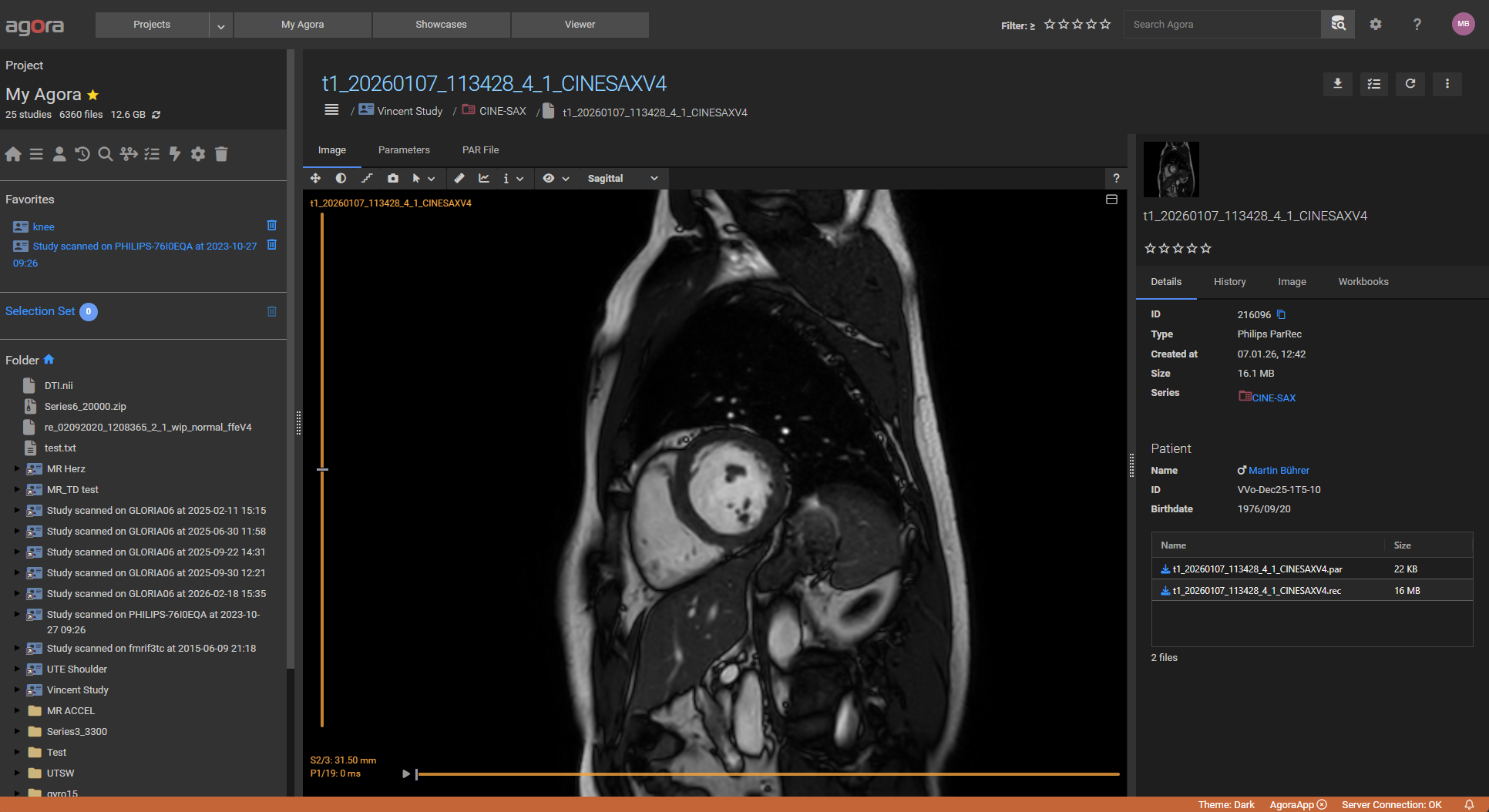
10.1. Single Viewer
The single viewer opens when you click a dataset’s preview image or the Open Viewer button in the data browser. It shows that one dataset in isolation.
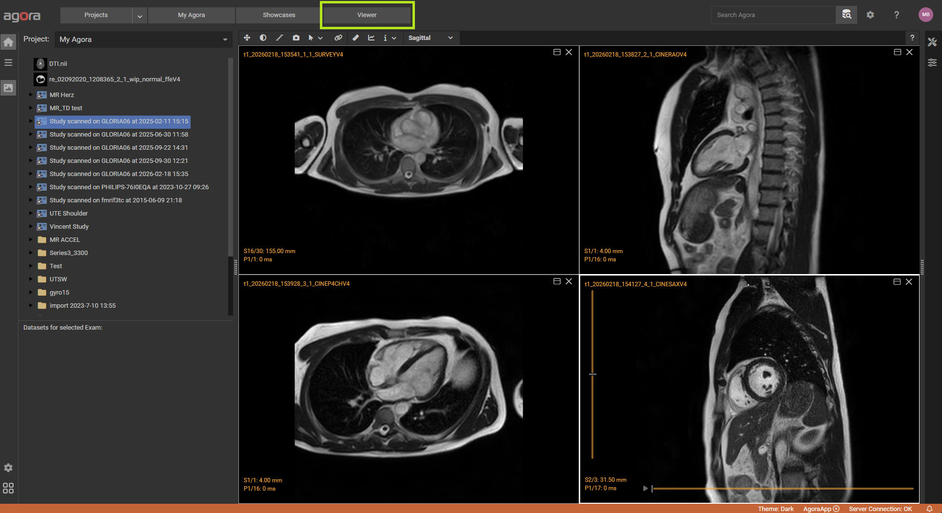
10.2. Multi-Viewer
The multi-viewer is accessed via the Viewer button in the main menu bar. It can display up to 9 datasets simultaneously in a configurable grid (up to 3×3). Datasets from different projects can be shown side by side.
To populate the multi-viewer, drag and drop a study, a series, or individual datasets into a viewer slot:
Study — the first n datasets of the study fill the available slots (in the order they appear in the data browser).
Series — the first n datasets of the series fill the available slots.
Dataset — the specific dataset is placed in the target slot.
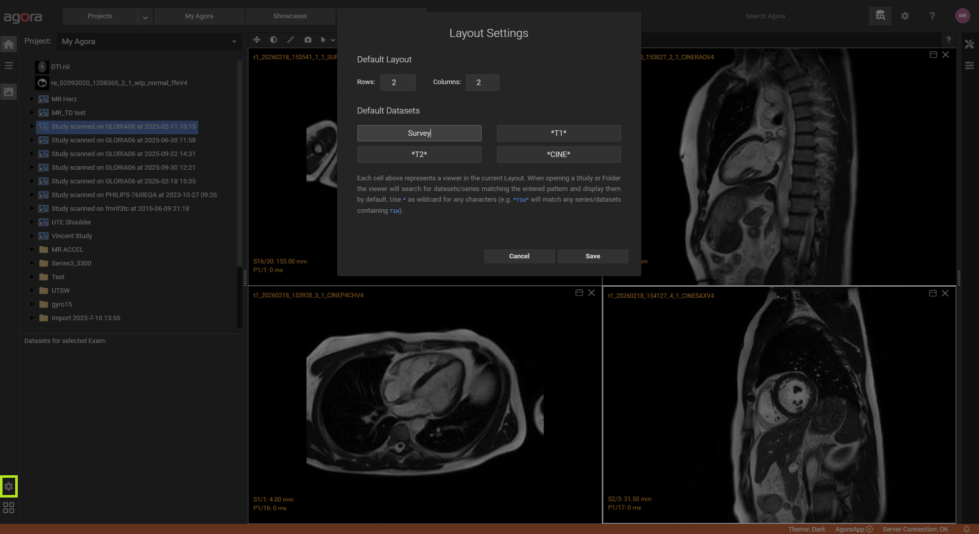
Naming patterns — the default first-n behaviour can be overridden per slot in the multi-viewer settings. Each slot can be assigned a naming pattern; the first dataset whose name matches the pattern is displayed in that slot. This is useful for always comparing the same dataset types across different studies — for example, always showing the T1, T2, and FA maps in the same layout regardless of the order datasets appear in the study.
10.3. Supported Formats
The viewer supports the following dataset types:
DICOM — standard medical imaging
NIfTI (NIfTI-1 and NIfTI-2)
Philips — PAR/REC, Raw MRI, Spectroscopy
Siemens Raw MRI
Bruker Raw MRI
ISMRMRD
VTK — surface and volume files (.vtk, .vti, .vtp, .stl) rendered in the 3D viewer
MR Spectroscopy — MRUI format and Philips spectroscopy
10.5. Toolbar

The toolbar at the top of each viewer pane provides the following controls:
Fit to Window — reset zoom so the image fills the available pane.
Reset Contrast — restore the window/level to its default value.
Interpolation — toggle smooth interpolation on/off (off = raw pixel display).
Snapshot — save the current view as a PNG image. In gallery modes the full grid is exported as a single image.
Mouse Mode — dropdown to set what left-click does: None, Zoom, Pan, or Contrast (window/level adjustment).
Link — synchronize slice position and/or time point with other open viewer panes (only available in the multi-viewer; see `Linked Viewers`_ below).
Show Contour / Show Mask / Show Statistics — toggle the visibility of contour overlays, mask overlays, and the statistics panel (visible only when a workbook is active).
Measure — draw a distance measurement on the image; the length and angle are displayed alongside the line.
Profile — draw a line across the image to extract an intensity profile along it.
Information — dropdown to toggle overlay information: slice number, pixel value under the cursor, and patient coordinate system.
Display Mode — dropdown to switch how slices are laid out (only available in the single viewer):
Single — one slice at a time (default)
Slice Gallery — all slices for the current time point arranged as a grid
Phase Gallery — all phases for the current slice arranged as a grid
Contrast Gallery — all contrasts arranged as a grid
The gallery modes are useful for quickly reviewing all slices of an acquisition or comparing cardiac phases.
Anatomical Plane — dropdown to switch between Sagittal, Coronal, and Transversal views (only shown for datasets with 3D orientation information).
Help — hover to display a keyboard shortcuts reference.
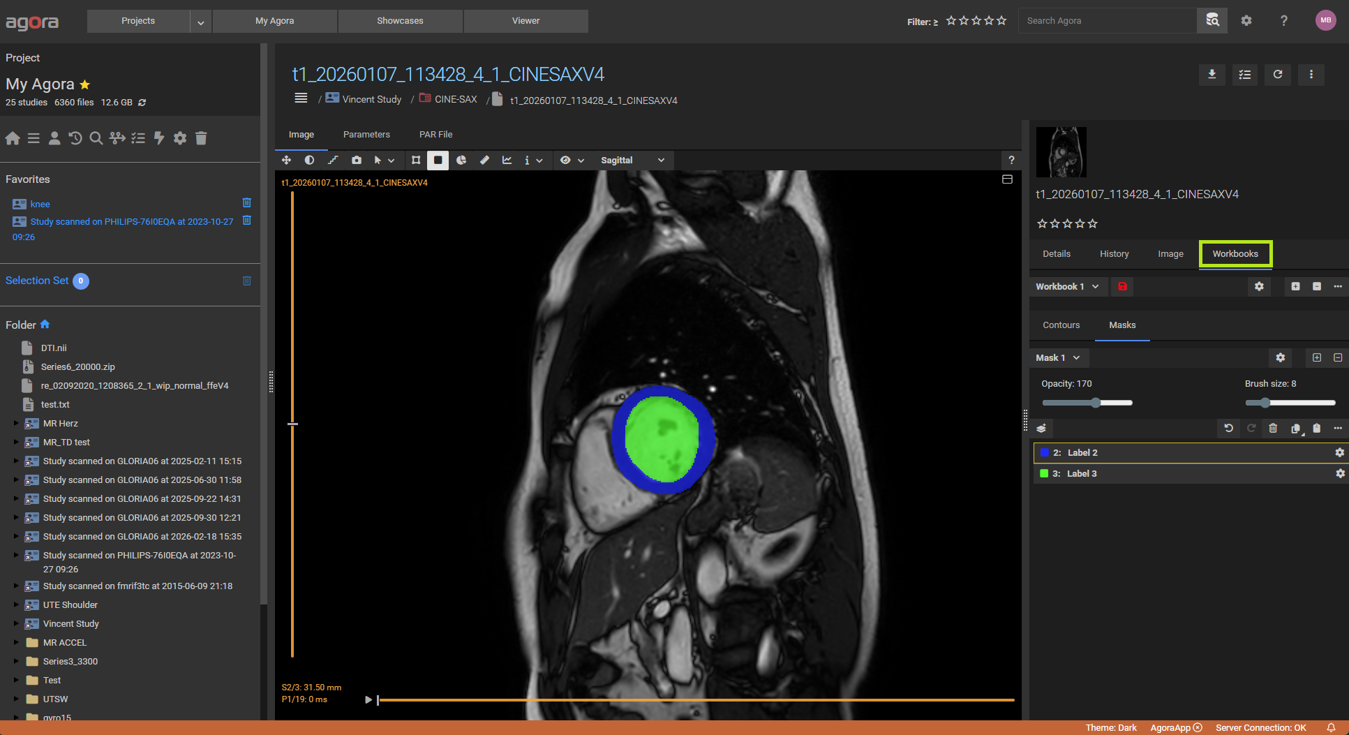
10.6. Workbooks
The workbook panel (open via the Workbook button) provides structured ROI and cardiac analysis on top of image data.
Workbook types:
ROI — general-purpose region-of-interest analysis
Cardiac MR (CMR) — pre-defined structures for cardiac analysis (LV/RV endo- and epicardium, pericardium, scar, MVO)
Generic / Template — custom templates for standardized protocols
Drawing tools — available in the Contour tab:
Polyline, Freehand, Circle, Rectangle, Spline
Contours can be 2D (per-slice) or 3D, and optionally time-invariant (propagated across all phases).
Masks — the Mask tab enables pixel-level segmentation with a brush tool. Up to 256 labelled regions are supported. Brush size and opacity are adjustable.
Statistics — the Statistics tab displays quantitative metrics (mean, SD, area, volume) computed from the drawn contours and masks.
Cardiac analysis (CMR workbooks) — the CMR tab provides:
LV function analysis (volumes, ejection fraction, mass)
Late enhancement analysis (scar quantification)
Perfusion and first-pass perfusion analysis
Undo/Redo — Ctrl+Z / Ctrl+Y (10-level history for contour and mask edits).
Keyboard shortcuts for workbook editing:
Shortcut |
Action |
|---|---|
|
Copy selected contour/mask |
|
Paste to current slice |
|
Paste to all slices |
|
Paste to all time points |
|
Select all contours on current slice |
|
Delete selected contour/mask |
|
Cancel current drawing action |
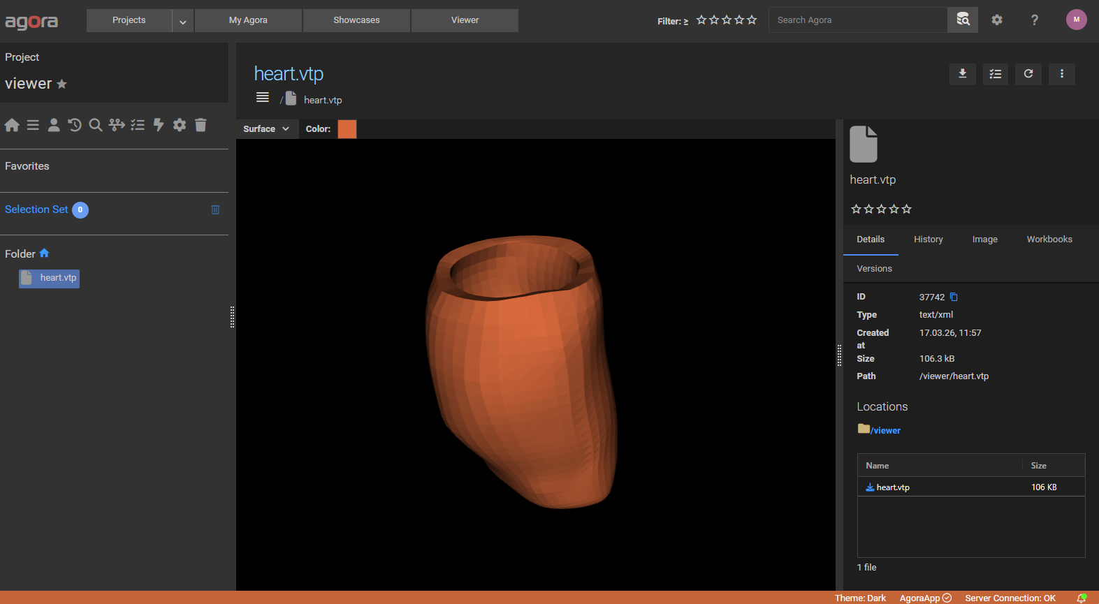
10.7. 3D Viewer
VTK datasets (.vtk, .vti, .vtp, .stl) open in the 3D viewer. Use the representation selector to switch between:
Surface — solid surface rendering
Wireframe — mesh edges only
Surface with Edges — combined
Slice — 2D cross-section through the volume
Points — point cloud
Left-click drag rotates the model; middle-click drag pans; mouse wheel zooms.
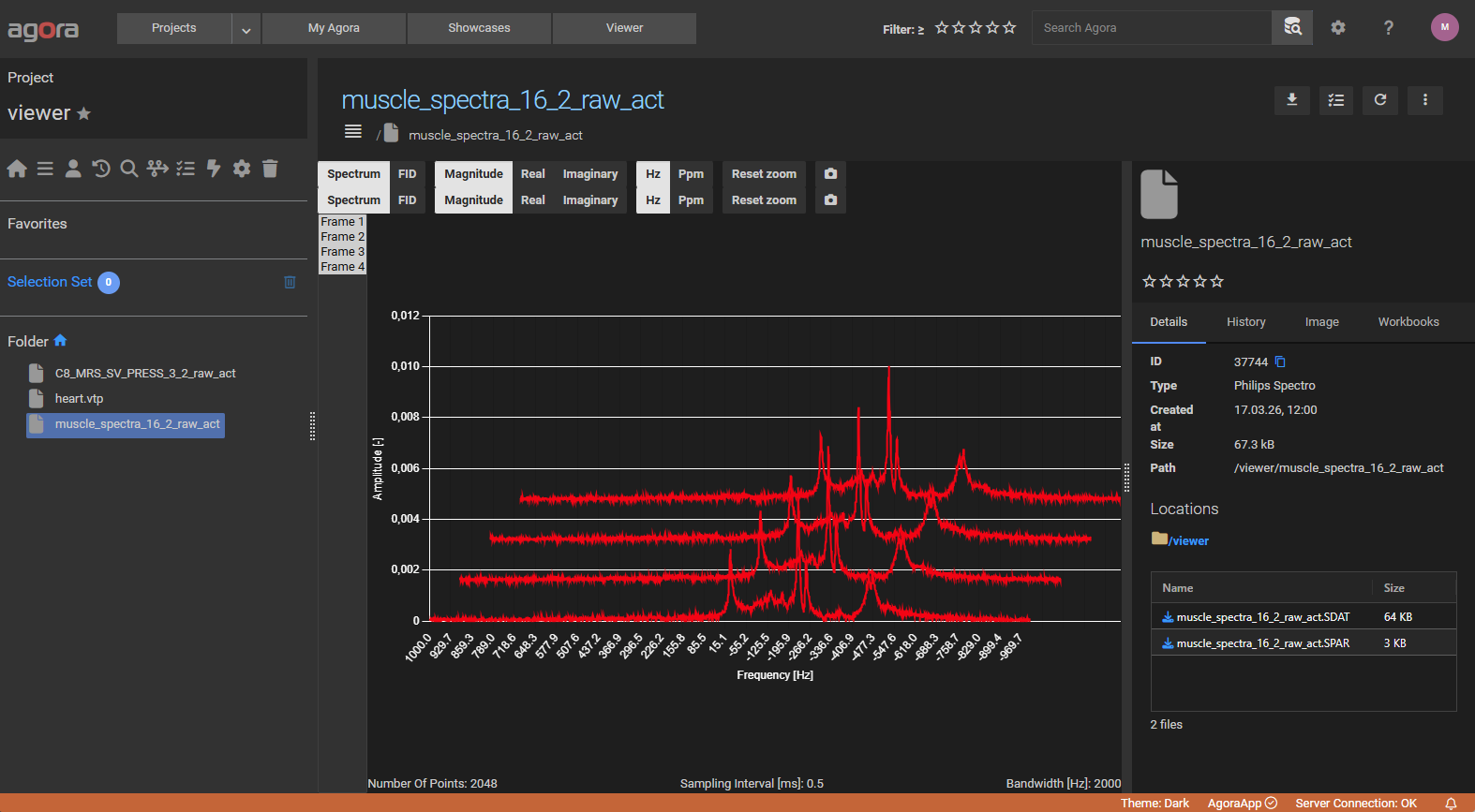
10.8. Spectroscopy Viewer
MR spectroscopy datasets open in a dedicated spectroscopy viewer that displays spectra as line graphs.
Switch between Magnitude, Real, and Imaginary signal representations using the toolbar.
Toggle the frequency axis unit between Hz and PPM.
Scroll through spatial positions to inspect individual voxel spectra.