2. Quick-Start Tutorial
Follow this tutorial for a quick start with GTFlow.
Step 1
Start the GTFlow application by double-clicking the GTFlow icon on your desktop or by using the standard program-start menu of your operating system.
2.1. Opening the built-in sample dataset
Step 2
On the start page in the ‘Getting Started’ box, select ‘Open small sample dataset’.
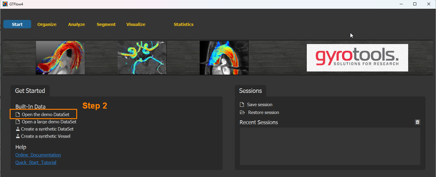
Figure 2.1: Opening the built-in sample dataset.
The built-in 4D-flow dataset is loaded to memory and is listed on the ‘Dataset Management’ box on the Organize page. The individual components of the flow dataset are assigned along with the respective flow-encoding values and the heart phase interval.
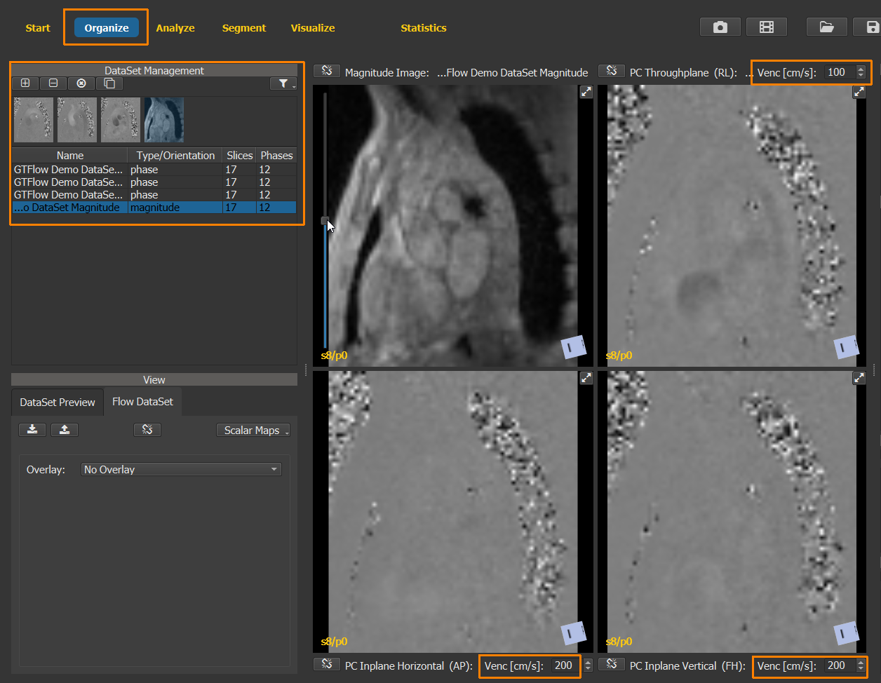
Figure 2.2: The Organize page with the flow dataset viewers.
To navigate through the slices, point to the left border of a viewer window to reveal the scroll bar. Use the time bar at the bottom of the page to navigate through the heart phases. Press the middle mouse button and move the pointer diagonally to change the image contrast. Use the mouse wheel or simultaneously press the left and middle mouse button to zoom the image in and out.
2.2. Overlay and masks
Step 3
In the ‘View’ box on the Organize page, select ‘In-Plane Velocity’ for the image overlay choice.
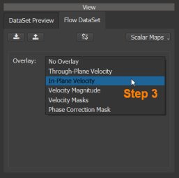
Figure 2.3: Selecting the display overlay of the flow dataset.
Step 4
In the ‘Velocity Field Mask’ box on the right of the Organize page, check the ‘Magnitude image intensity threshold’ box to enable the corresponding velocity field mask. Adapt the threshold value to 150.
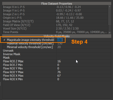
Figure 2.4: Enabling the magnitude intensity mask and setting the threshold.
Velocity field mask operate on a voxel level. In every masked voxel, all velocity components of the velocity field are set to zero. Multiple masks can be active at the same time and only voxels which are not masked by any of the active masks keep their original velocity values. Masks should be applied with caution when deriving quantitative values in GTFlow. If voxels inside a blood vessel are masked, the calculated flow values in that vessel will be affected.
Step 5
In any of the viewer windows, press Ctrl + left mouse button and drag the pointer. This defines a main ROI mask.
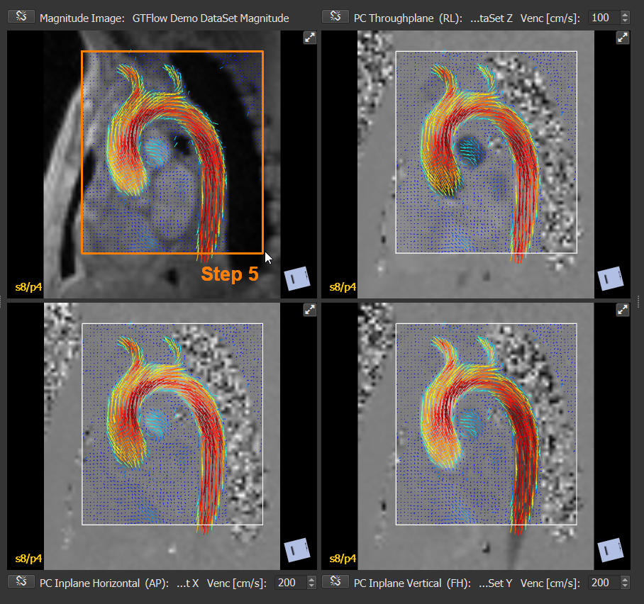
Figure 2.5: Interactive definition of the main ROI mask.
The main ROI mask will limit the size of the flow field to the selected region. Use this feature when working with large datasets. It will save memory and shorten subsequent processing time. To remove a main ROI mask, double-click in the viewer window.
2.3. Analyze page
Step 6
Switch to the Analyze page by selecting the page in the main application tool bar.
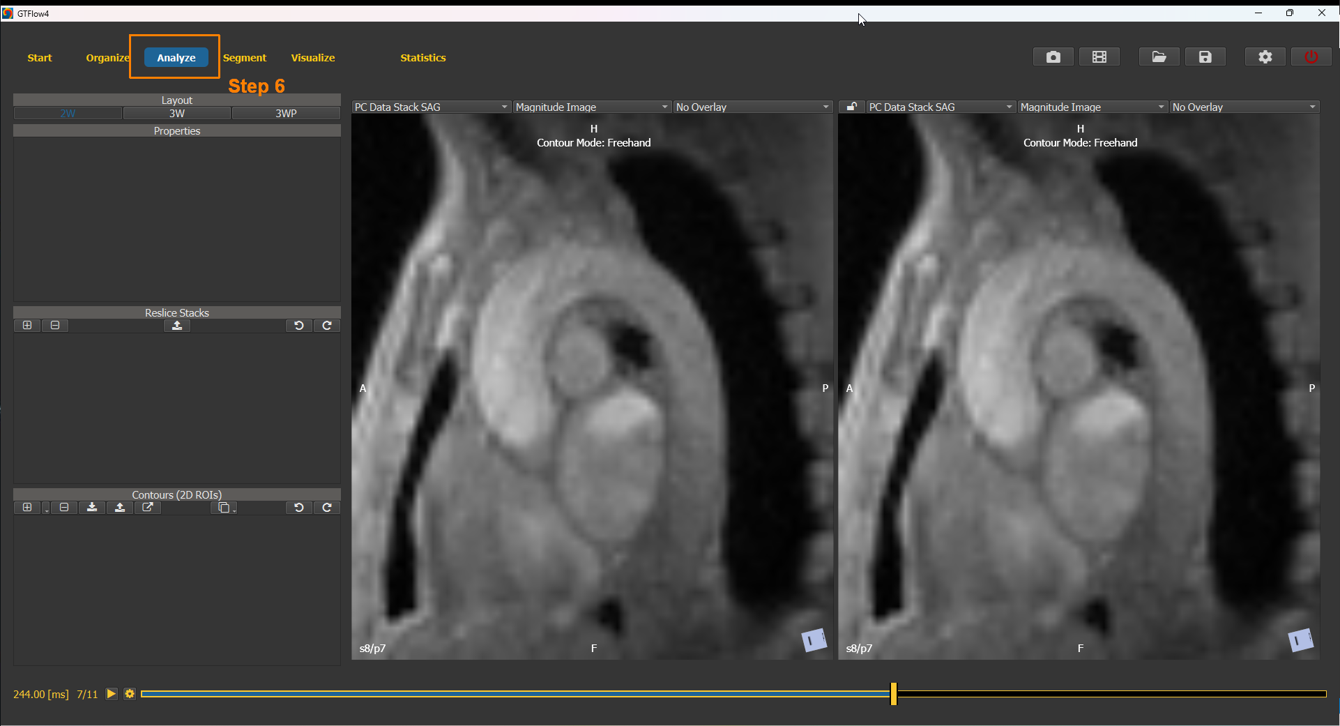
Figure 2.6: The Analyze page with the configurable side-by-side viewers.
The Analyze page features two or three side-by-side viewers, which can be individually configured with respect to stack orientation, displayed dataset, and overlay. The Analyze page is used for the 2D-segmentation of blood vessels using contours and to analyze flow values. To that end, the image stack of the flow dataset can be re-sliced (reformatted) in arbitrary orientations.
2.4. Defining a reslice stack
Step 7
In the ‘Reslice Stacks’ box use the ‘+’ button to create a new reslice. Use the stack planing handle to create a reslice image perpendicular to the vessel of interest (in this dataset the aortic arch).
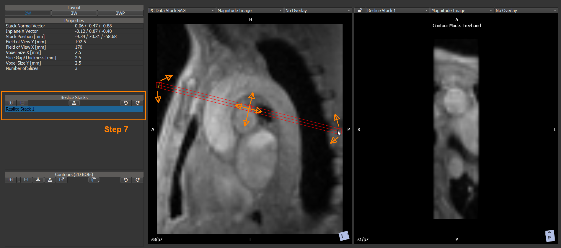
Figure 2.7: Creating and positioning a reslice stack.
2.5. Defining vessel contours
Step 8
Configure the viewer with the reslice stack to display the ‘Inplane Y PC image’. Using the time bar, advance to a systolic heart phase with high velocities in the aortic arch (eg 139ms).
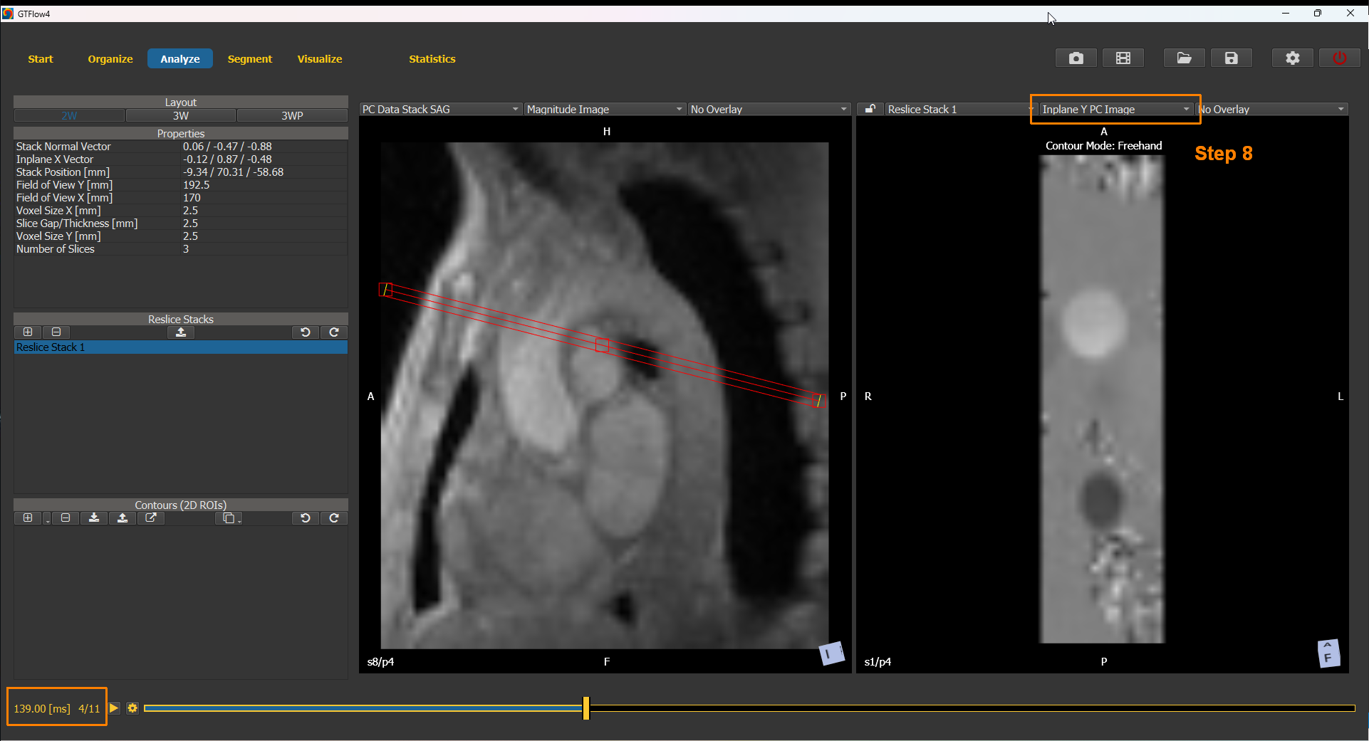
Figure 2.8: Preparing the view for contour drawing .
Step 9
In the ‘Contours’ box use the ‘+’ button to create a new contour. In the window with the reslice stack, pressing the left mouse button, draw a contour around the ascending aortic cross-section. Repeat to draw a second contour around the descending aortic cross-section.
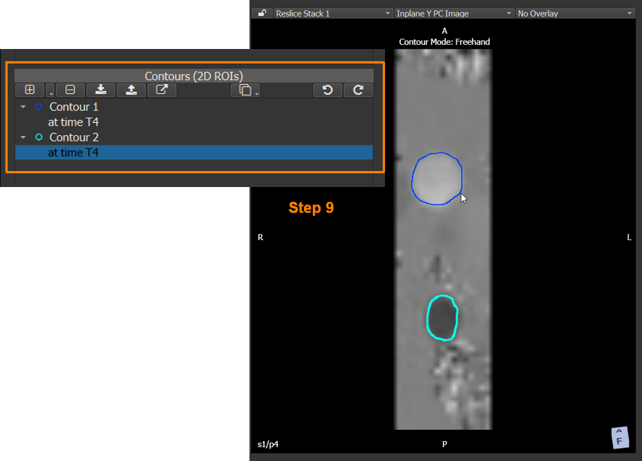
Figure 2.9: Adding and drawing contours.
2.6. Flow Statistics
Step 10
Open the Statistics panel by selecting it on the main application tool bar. On the Statistics panel, make sure that the ‘Contour Statistics’ tab and the ‘Flow’ statistics category are selected. The contour table will display the previously defined contours along with the corresponding flow values.
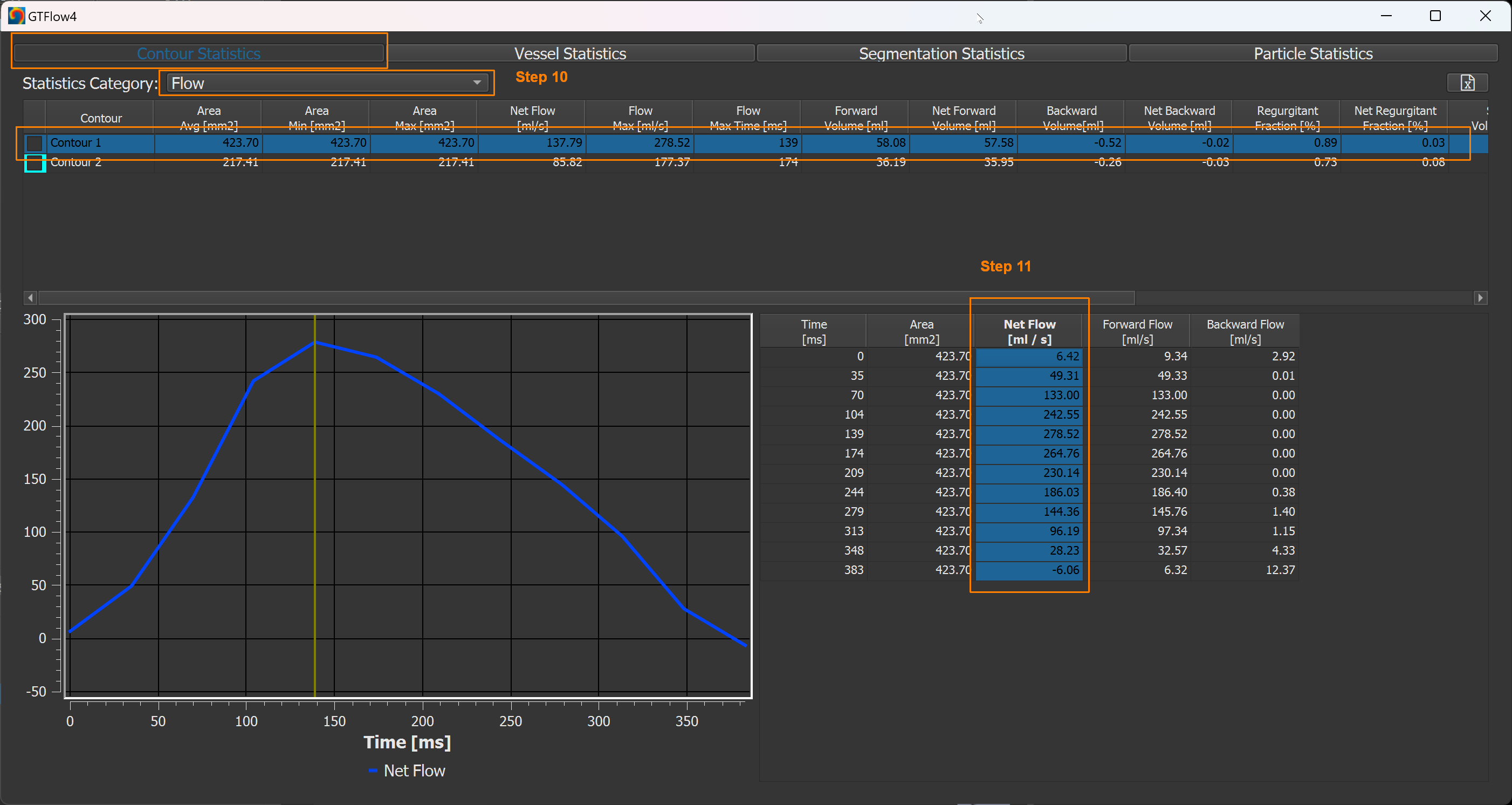
Figure 2.10: Table selection in the statistics panel.
Step 11
In the contour table on the Statistics panel, select a contour by left-click anywhere on a table line. The lower right time-resolved statistics table will be populated with the individual statistics for each heart phase. Select on or more columns in the time-resolved statistics table to get a graphical representation of the values over time.
2.7. Scene viewer
Step 12
Switch to the Visualize page by selecting the page in the main application tool bar.
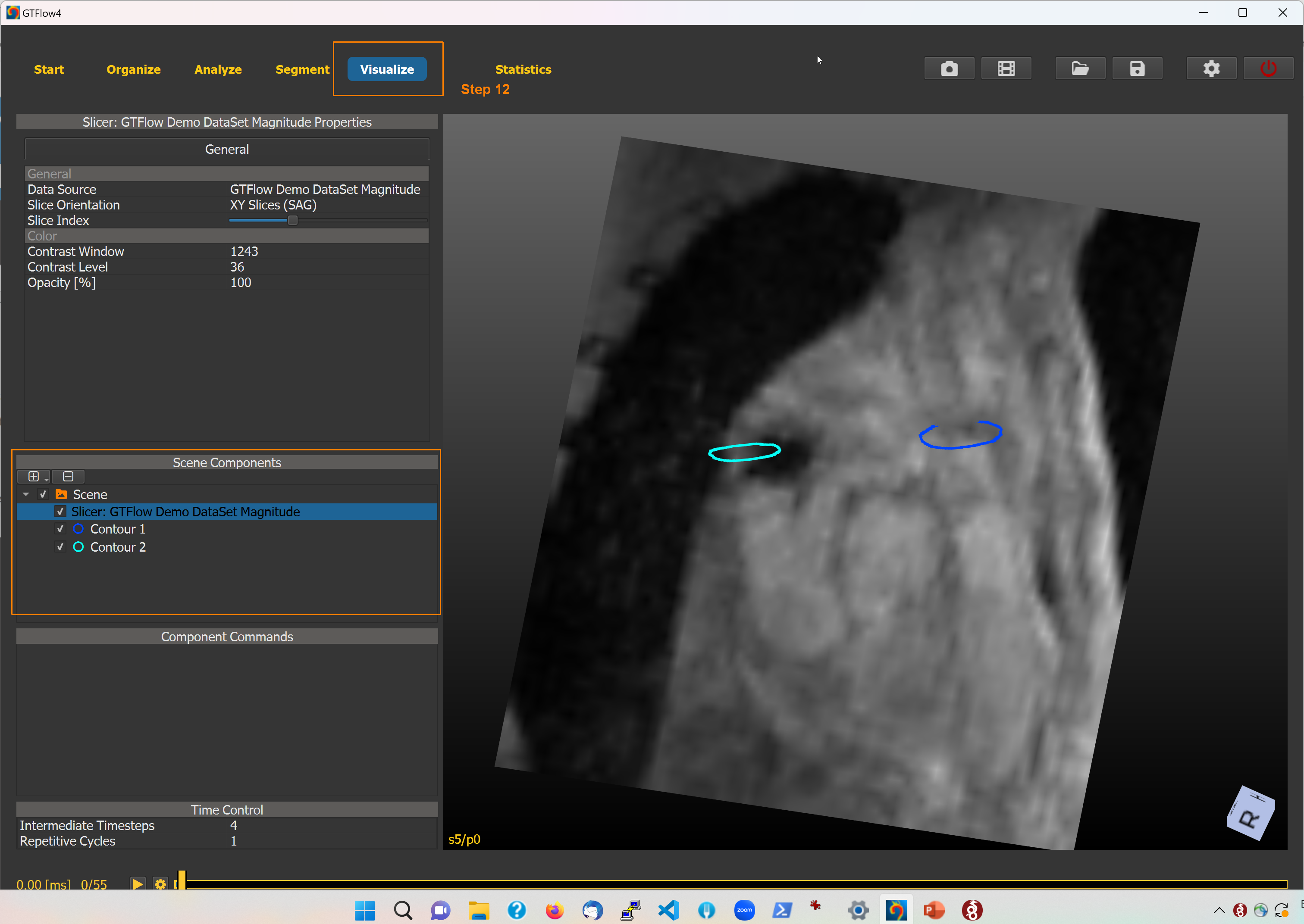
Figure 2.11: The Visualize page with the scene viewer and the scene components.
The Visualize page displays a 3D scene viewer. The scene displayed can be configured by adding scene components to the scene graph. The current scene components are listed in the “Scene Components” box. Selecting an individual component in the list displays the configurable component properties in the “Properties” box. At this time of the tutorial, four scene components have already be added to the scene graph: A top-level folder component, and orthogonal slice component and two contour components representing the previously drawn contours.
To reorient the scene, use SHIFT-CTRL and the left mouse button. Use the mouse wheel to zoom the scene in an out.
2.8. Generating pathlines
Step 13
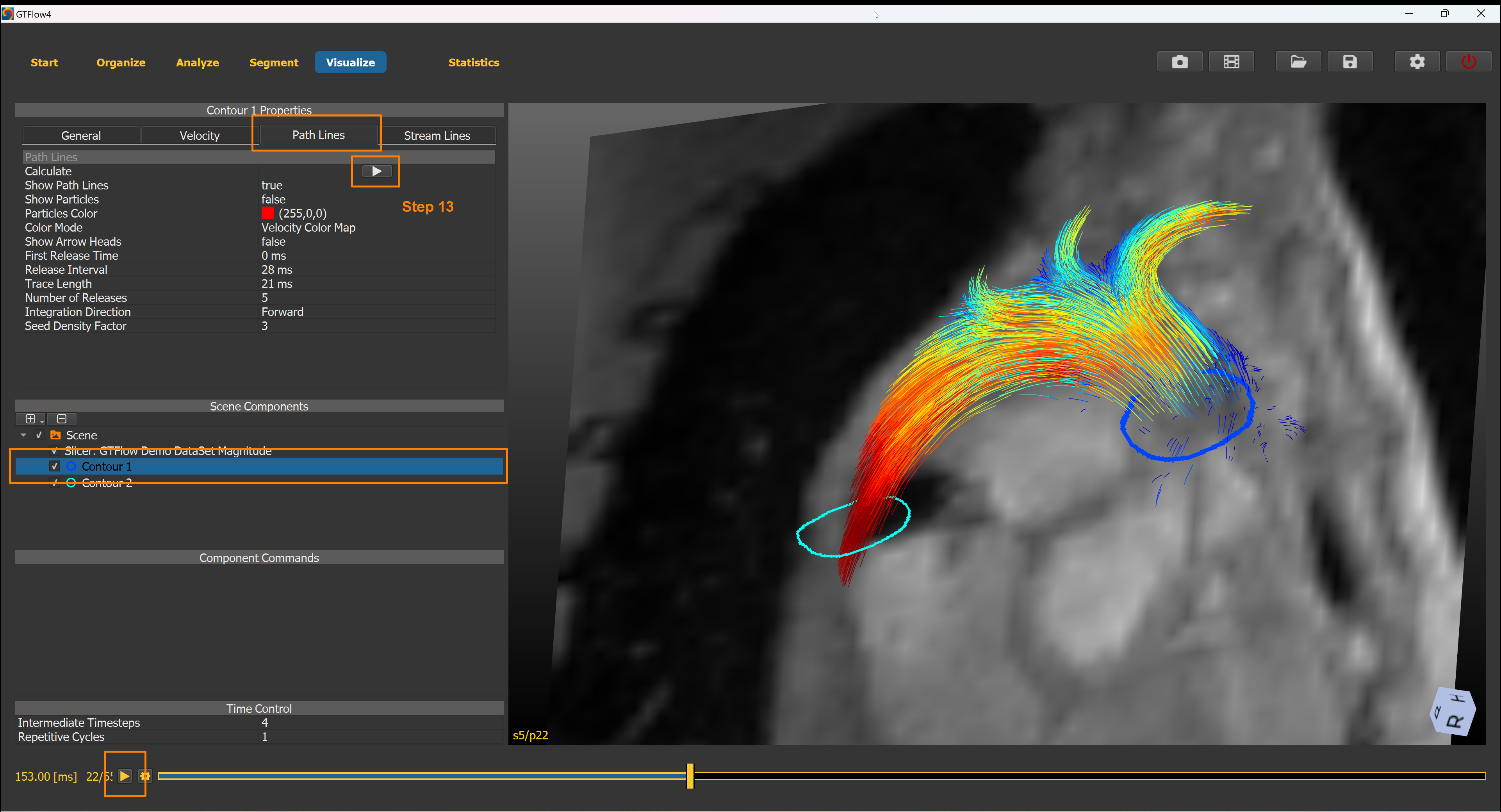
Figure 2.12: Generating velocity field pathlines from seed points within a contour.
2.9. Save session
Step 14
On the main application tool bar use the ‘Save session to file’ () button to save the current state of GTFlow to a session file on disk. The session can be restored from this file at any later time.
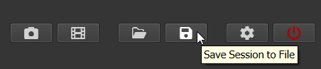
Figure 2.13: Saving a session to file for later use.