3. Overview

3.1. The Main Toolbar

Figure 3.1: The main application toolbar.

The GTFlow application is structured over several functional pages, which can be selected on the main toolbar at the top of the application. The toolbar also provides access to the program settings and to the quick-access menu.

3.2. The Start Page

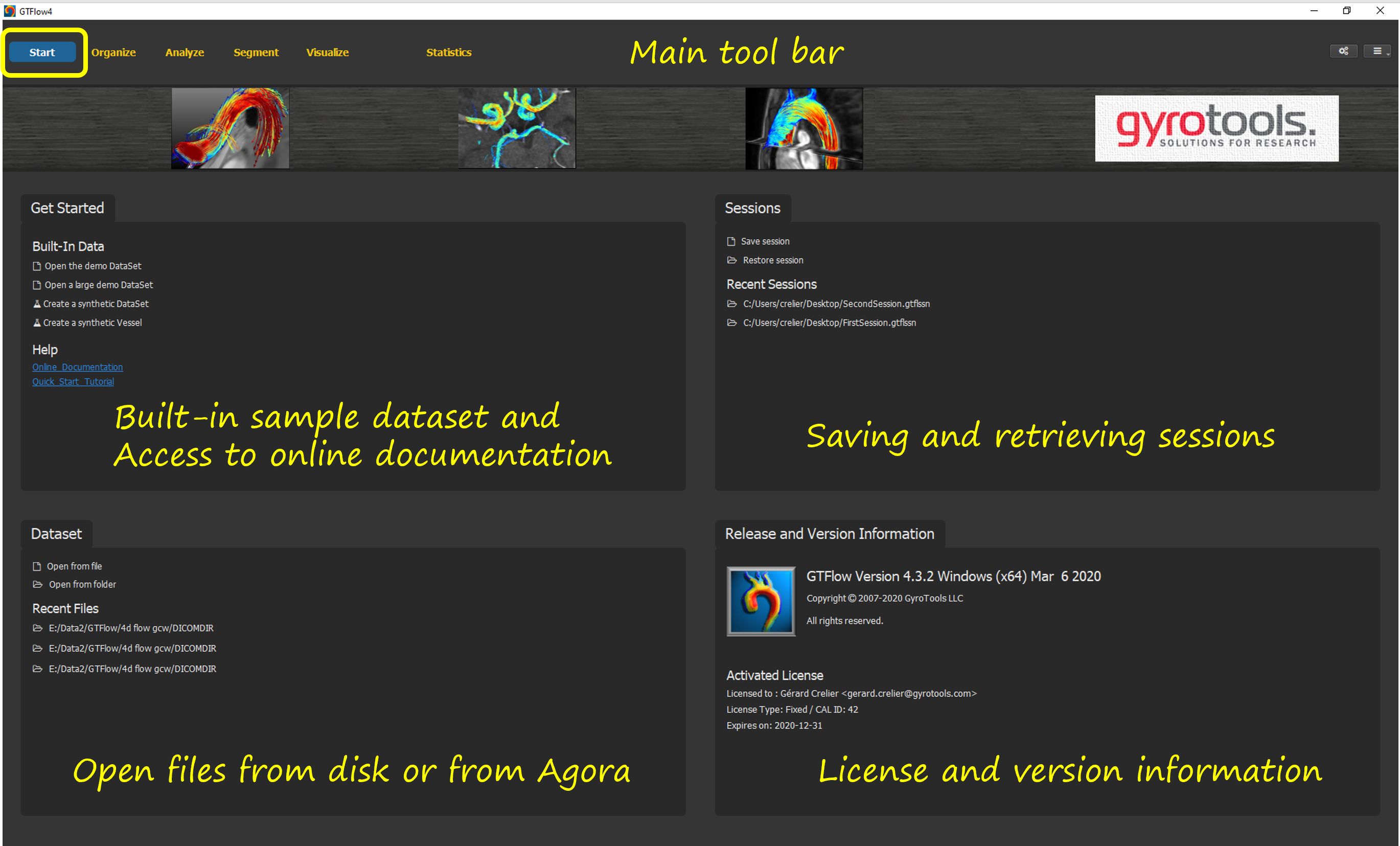
Figure 3.2: The Start Page.

When launching the GTFlow application, the Start Page is displayed. Here data files and session files can be opened from disk. Also lists of recently used files and sessions are displayed for quick access. The start page also provides links to the documentation, to the built-in demo dataset, and to the synthetic data generator. Finally, version and license information is displayed in the lower right box.

3.3. The Organize Page

Figure 3.3: The Organize Page.

The Organize Page provides the functionality to load and pre-process datasets, as well as to aggregate them into a flow dataset. The flow dataset consists of a magnitude and 3 velocity encoded phase datasets along with the velocity encoding factors that define the velocity field. When loading files, GTFlow will attempt to populate the flow dataset automatically. The configuration however can also be set manually. The controls on the right of the organize page allow to mask the velocity field of the current flow dataset using any combination of implicit or explicit voxel masks. In addition, the velocity field can be corrected for phase offsets typically resulting from eddy currents during acquisition. Phase aliasing due to inadequate velocity encoding strengths can also be corrected for.

The Time Control Bar at the bottom of the page allows to scroll through the individual heart phases of the currently displayed dataset. A time animation mode allows to continuously loop through the heart phases.

In any viewer on the Organize Page, pressing Ctrl + left mouse button and dragging defines a main ROI mask that restricts the active flow field to a rectangular sub-region. This reduces memory usage and speeds up all downstream processing. Double-click in the viewer to remove the ROI mask.

3.4. The Analyze Page

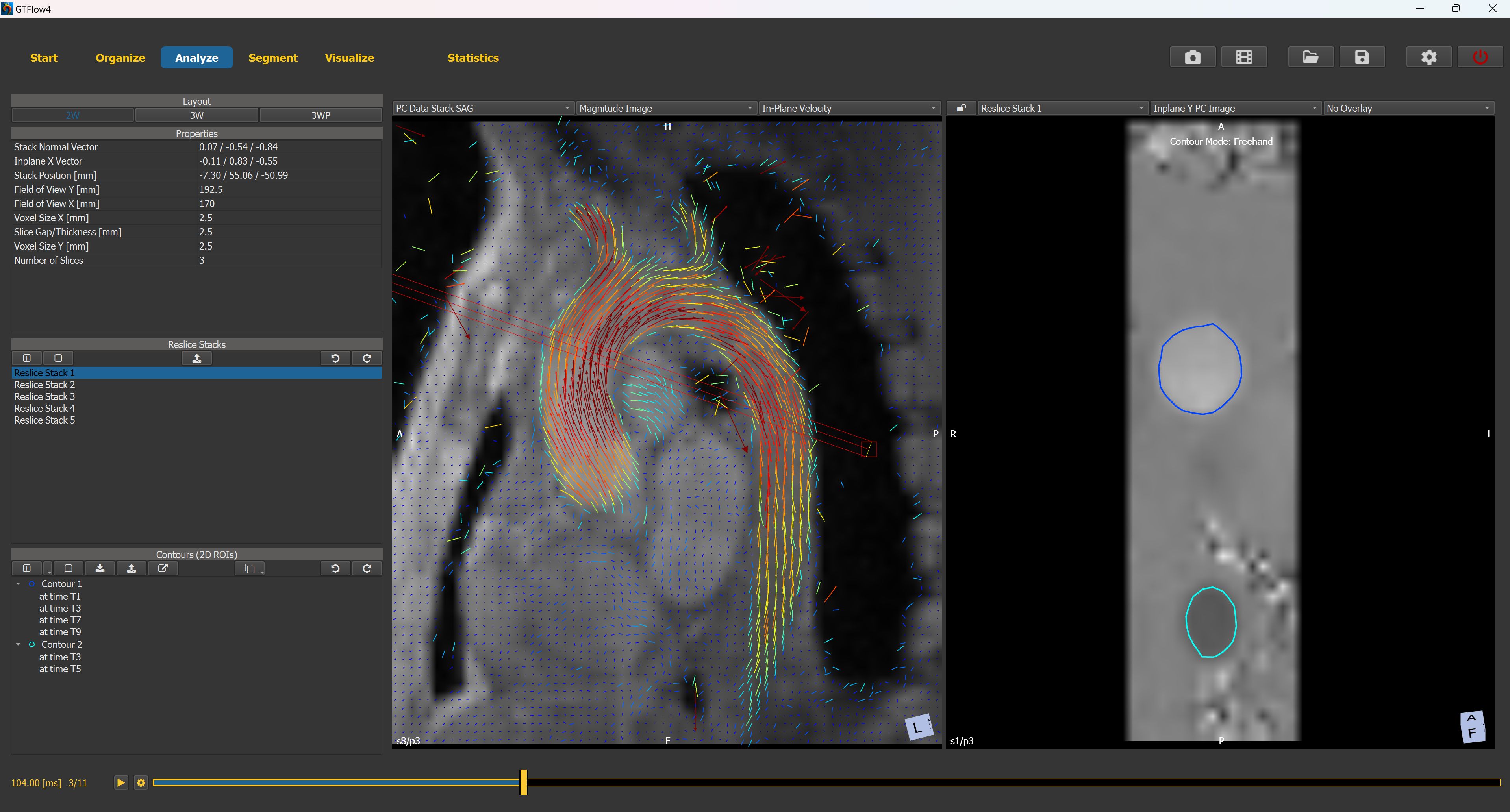
Figure 3.4: The Analyze Page.

The Analyze Page has two or three side-by-side windows which can be individually configured to display any of the components of the flow dataset in any available native or resliced orientation. Various color overlays can also be configured.

The controls on the left of the page allow to generate an arbitrary number of image reslice stacks from the current flow dataset. The main purpose of reslice stacks is to obtain an image plane perpendicular to the blood vessel of interest. Once such a view is available, the vessel can be manually segmented by contouring the lumen of the vessel with a contour. A contour has a representation in each heart phase and can be adapted to a vessel lumen or position change over time. However, drawing a contour in each heart phase is optional. In any heart phase with no contour representation, the contour closest in time will be used.

Contours defined on the analyze page will also be visible on the visualize page. Velocity and flow statistics of each contour will be listed on the statistics page.

3.5. The Segment Page

Figure 3.5: The Segment Page.

The Segment Page is used to create and edit 3D segmentation masks, generate vessel surface meshes, and manage vessel objects.

The page is organized around three main areas:

• Segmentation Management (left panel) — contains three stacked tables for Masks, Labels, and Commands. A mask defines the spatial extent of a segmentation. Each mask can hold one or more labels (colored regions), and each label can have one or more commands applied to it to assign voxels.

• Viewers (center) — up to four synchronized viewer panels are shown: three orthogonal 2D slice views (XY, YZ, XZ) and one 3D volume view. An additional vessel viewer is shown when a vessel object is selected. Use the expand button in any viewer to maximize it.

• Vessel List (right panel) — lists all vessel surface meshes. Vessel commands for surface smoothing, center line generation, contour creation, and segment creation are accessed here.

Figure 3.6: Mask and label management on the Segment Page.

Creating a segmentation follows four steps:

1. Click + in the Masks table to create a new 3D or 4D mask. Select a dataset to define the mask dimensions.

2. A default label (Label 1) is created automatically. Add further labels with + in the Labels table.

3. Add a command to a label using + in the Commands table and select a command type from the dropdown.

4. Interact with the active command in the viewer panels to assign voxels to the label.

Figure 3.7: Active command with its Settings and Help tabs.

The active command is displayed in an expandable panel below the Commands table, showing Settings and Help tabs. All commands support undo/redo.

Creating a vessel from a label: Once a satisfactory segmentation exists, select a label and click the Create Vessel button in the Vessel List panel. The resulting surface mesh can be further refined with the surface smoothing and decimation commands.

3.6. The Visualize Page

Figure 3.8: The Visualize Page.

The Visualize Page provides an interactive 3D scene viewer for rendering and animating all application objects together. It is composed of three areas:

• Scene Components (left panel) — a tree of all nodes currently in the scene. Use the + (Add) button to insert new nodes. Each node has a visibility toggle and can be reordered by drag-and-drop.

• 3D Viewer (center) — an OpenGL scene rendered in real time. Rotate with Ctrl+Shift + left mouse button, zoom with the mouse wheel, and pan with middle + right mouse buttons.

• Properties (right panel) — shows the configurable properties of the currently selected scene node. Properties are organized in tabs (General, Wall Shear Stress, Path Lines, etc.) depending on node type.

Figure 3.9: Scene graph with multiple scene node types.

Available scene node types:

Node type	Description
Slice	An orthogonal or oblique image slice plane
Reslice	A user-defined reslice stack plane
Contour	A 2D analysis contour (from the Analyze page)
Vessel	A 3D vessel surface mesh with optional WSS coloring
Vessel Segment	An individual segment of a vessel
Velocity	A velocity vector field visualization
Path Lines	Computed velocity path lines from a seed contour
Stream Lines	Continuous stream line visualization
Wall Shear Stress	WSS color map draped on a vessel surface
Group / Folder	Container for organizing nodes

Keyframe animation allows the camera orientation, scene node visibility, and other properties to be interpolated over time to produce smooth flythrough animations.

Figure 3.10: The keyframe time bar at the bottom of the Visualize Page.

The Keyframe Time Bar is shown at the bottom of the page. Add keyframes at any time point, adjust scene and camera state for each keyframe, and GTFlow will interpolate between them. Use the Create Movie button in the toolbar to export the animation to a video file.

3.7. The Statistics Page

Figure 3.11: The Statistics Page.

The Statistics Page is a floating panel that can be opened from the main toolbar while any other page is active. It provides quantitative analysis of the velocity field for all contours, vessel objects, and segmentation masks defined in the session.

The page contains four tabs:

Contour Statistics

Figure 3.12: Contour Statistics tab.

Displays statistics computed inside 2D analysis contours. Select a category from the Statistics Category dropdown:

• Flow — net flow, forward flow, backward flow, and regurgitant fraction per contour per heart phase.

• Velocity — mean, peak systolic, and through-plane velocity values inside the contour.

• Generic — pixel-by-pixel values of any loaded dataset sampled inside the contour.

The upper table shows one row per contour with aggregate values across all heart phases. The lower table shows time-resolved values for the selected contour. Select one or more columns in the lower table to generate a time plot.

Vessel Statistics

Figure 3.13: Vessel Statistics tab.

Displays statistics computed on 3D vessel objects and their segments. Categories include:

• Velocity — mean velocity, peak velocity, and flow rate over the vessel or per segment.

• Wall Shear Stress — requires a WSS calculation to have been completed (see Assessing Wall Shear Stress).

• Pulse Wave — pulse wave velocity analysis; requires vessel segments and a center line.

• Generic — values of any dataset sampled within the vessel volume.

Segmentation Statistics

Displays statistics computed inside a segmentation label volume. Categories include Velocity and Generic (any loaded dataset).

Particle Statistics

Displays results of particle transport analysis between emitter and target contours or vessel segments. See Particle Statistics for the full workflow.

3.8. The Time Axis and Time-Resolved Objects

3.8.1. The Time Axis

The time axis in GTFlow represents the cardiac phases of the loaded 4D flow dataset. Each phase is stored as an absolute time value in milliseconds measured from the start of the cardiac cycle (trigger point). The number and spacing of these phases depend entirely on the acquisition: phases are not required to be equidistant, and the interval between consecutive phases can vary.

The cardiac cycle duration is a separate quantity from the individual phase times. It represents the total length of one complete heartbeat in milliseconds and is typically detected automatically from the acquisition parameters. It can be inspected and corrected on the Organize Page in the Flow Dataset tab. The cycle duration is used by GTFlow to correctly handle lookups that cross the cycle boundary (see below).

Note

The phase times and the cardiac cycle duration are detected automatically when loading a study. If the detected values appear incorrect, they can be adjusted manually on the Organize Page before proceeding with analysis.

3.8.2. Sparse Representation of Time-Resolved Objects

Contours, vessel geometries, and reslice stacks are all time-resolved objects: they can, but do not have to, carry a separate shape for every heart phase. GTFlow stores only the shapes that the user explicitly defines — the representation on the time axis is sparse.

At any displayed time point, GTFlow determines the shape to use by the following rule:

1. If a shape is defined exactly at the requested time, that shape is used.

2. Otherwise, the shape defined at the nearest earlier time point is used.

3. If no shape exists before the requested time (i.e., the requested time is earlier than all defined shapes), the first available shape in the cycle is used — wrapping around the cardiac cycle boundary using the cycle duration.

This means that drawing a contour in only one heart phase is sufficient for a valid analysis: GTFlow will use that single contour for all time points in the cycle. Adding contour representations at additional phases increases accuracy for vessels whose lumen or position changes significantly over the cardiac cycle.

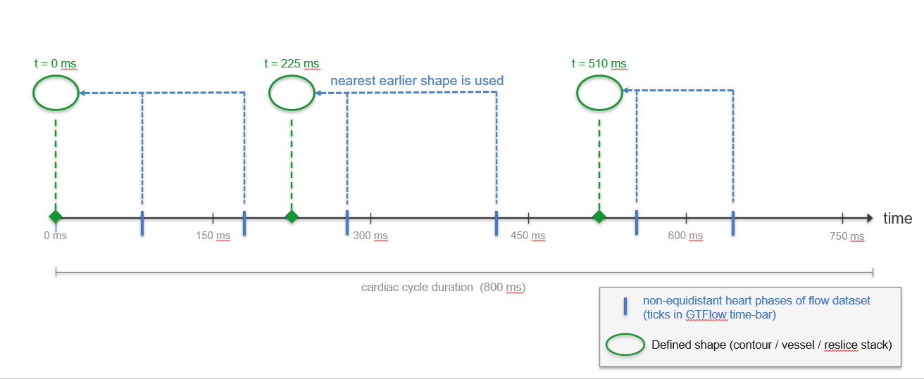
Figure 3.14: Illustration of the sparse time-resolved lookup rule. The shape defined at the nearest earlier time point is used at any queried time.

3.8.3. Vessel Shapes at Off-Axis Time Points

Vessel mesh geometries can be assigned to time points that do not coincide with any phase of the flow dataset. This is particularly useful when the vessel surface mesh was derived from a separate acquisition — for example, a 3D MR angiography scan acquired at a cardiac delay not present in the 4D flow phase list. In such cases, the mesh can be assigned to the time point of the MRA acquisition, and GTFlow’s nearest-earlier lookup will automatically map it to the correct range of flow phases.

To assign a vessel geometry to a specific time point, use the vessel geometry commands on the Segment Page after importing or creating the mesh.

3.9. Mouse and Keyboard Controls

Image display can be controlled in each viewer window individually. Move the mouse cursor inside a viewer window and use the following mouse and keyboard controls:

3.9.1. 2D Viewer

Function	Control
Context Menu	right mouse button
Zoom	middle+left mouse buttons or mousewheel
Reset zoom	context menu -> Fit to window
Pan	middle+right mouse buttons
Contrast	middle mouse button
Reset contrast	context menu -> Reset window/level
Select voxel	<Shift> + left mouse button

3.9.2. Contour Editing (Analyze Page)

Function	Control
Draw contour	left mouse button (A contour must be selected in the contour list)
Close contour	double-click left mouse button (in B-Splines and Polygon drawing modes)
Select contour	<Ctrl> + left mouse button inside contour, or double-click in contour list
Deselect contour	<Ctrl> + left mouse button outside contour
Edit selected contour	left mouse button
Delete contour vertex	<Shift> + left mouse button on vertex (in B-Splines and Polygon drawing modes)
Delete selected contour	delete button in contour list command bar
Copy selected contour	copy buttons in contour list command bar
Move selected contour	<Alt> + left mouse button
Move all contours	<Alt-Shift> + left mouse button
Draw iso contours	<Shift-Ctrl> + left mouse button (in Freehand, B-Splines and Polygon drawing modes)
Undo contour editing	undo button in contour list command bar
Redo contour editing	redo button in contour list command bar

3.9.3. Segmentation Commands (Segment Page)

Function	Control
Set seed point / apply brush	<Ctrl> + left mouse button
Disconnect / erase voxels (Region Grow)	<Ctrl> + left mouse button
Resize brush circle	<Ctrl> + mousewheel
Navigate slices	up / down arrow keys (in 2D viewers)
Maximize / restore viewer	expand button (upper-right corner of viewer panel)
Undo command step	undo button in command panel
Redo command step	redo button in command panel

3.9.4. 3D Scene Viewer (Segment + Visualize Pages)

Function	Control
Context Menu	right mouse button
Zoom	middle+left mouse buttons or mousewheel
Reset zoom	context menu -> Fit to window
Pan	middle+right mouse buttons
Rotate	<CTRL-Shift> + left mouse button