Geometry Transformations

Coordinate systems

There are different coordinate systems on the scanner and in MRecon, each serving a certain purpose. In the following sections we will take a detailed look at these coordinate systems and describe the transformations between them. The name for the coordinate system in MRecon is thereby given in quotes (e.g. ‘MPS’)and the units of the coordinates are given in square brackets (e.g. [mm]).

Image based coordinate systems

We basically divide the different coordinate systems into two groups: Image based systems and fixed systems. Image based systems are bound to the imaging volume and are dependent on angulation, offcentre, image orientation, fold-over direction, fatshift direction etc. They can either be right or left handed. In MRecon we differentiate between three image based systems:

Matrix coordinate system ‘ijk’ [pixel]

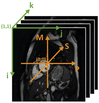
The coordinates in the matrix coordinate system basically specify a matrix index into the imaging data (r.Data) in Matlab notation. Meaning that the origin is located in the upper left corner of the image and starts with (1,1). The first axes runs along the vertical image axes from top to bottom, the second along the horizontal axes from left to right and the third one runs through the imaging volume from front to back (see image below). If the RotateImage function has not been called yet, the first axis corresponds to the readout direction while the second and third axes correspond to the phase encoding directions. After the RotateImage function the ‘ijk’-system is identical to the ‘REC’-system (see below). The units of the coordinates are given in pixels. This coordinate system can for example be used if one wants to know where a voxel in r.Data is located in the patient’s body or if ROI’s defined on different scans are transformed into the same system (transformation from ‘ijk’-system to ‘RAF’ or ‘xyz’-system).

MPS coordinate system ‘MPS’ [mm] / ‘MPSpix’ [pixel]

The ‘MPS’-system is very similar to the ‘ijk’-system but its origin lies in the center of the imaging volume and starts with (0,0). The first axes of the ‘MPS’-system runs along the readout direction of the image while the second and third axes run along the phase encoding directions. Before the RotateImage function has been executed the M-axis is parallel to the i-axis, and the P/S-axes are parallel to the j/k-axes in MRecon. After the RotateImage function the orientation of the MPS-axes depend on the scan parameter, such as orientation, fold-over direction, fatshift direction etc. The units of the MPS-system are either in mm (‘MPS’) or in pixel (‘MPSpix’).

REC coordinate system ‘REC’ [pixel]

The ‘REC’-system defines the orientation of the image as it is displayed on the scanner console. Its coordinates are given in pixel and its origin is in the upper left corner of the image (the same as in the ‘ijk’ -system). The RotateImage function is basically a transformation from the MPS-system to the REC-system and rotates/flips the imaging volume such that it is aligned in the same way as on the scanner console. After the RotateImage function the ‘ijk’-system is identical to the ‘REC’-system. The REC system only depends on the image orientation (transversal, coronal, sagittal) but is independent of the fold-over direction and fatshift direction.

Fixed coordinate systems

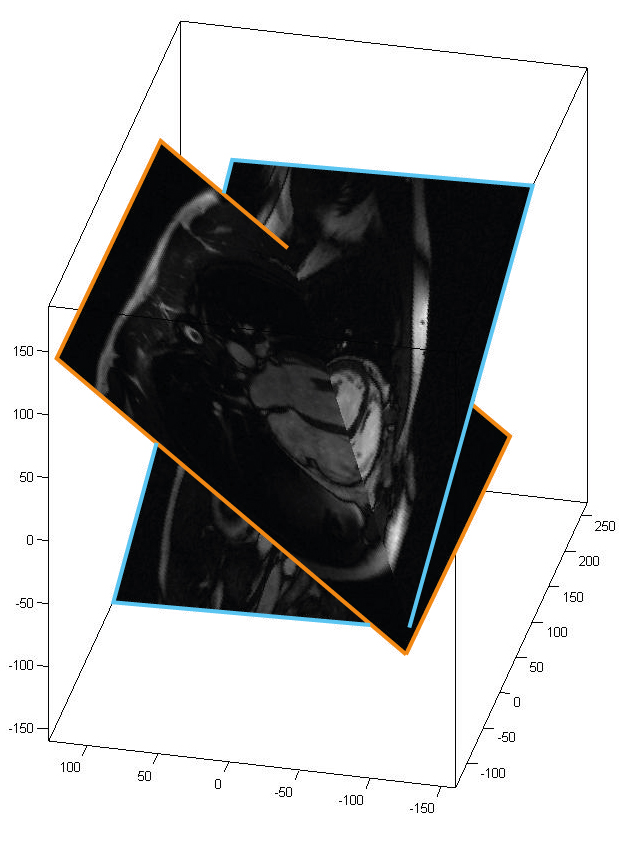
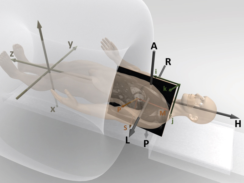
Fixed coordinate systems are independent on the imaging volume and are either bound to the patient (patient-system ‘RAF’) or the Scanner (scanner-system ‘xyz’). Fixed systems can be used to transform coordinates or imaging volumes from different scans into an identical system (e.g. plot imaging slices from different scans in 3D). In the image on the right a cardiac short axes view is plotted together with a long axes view by transforming the images from the image based ‘ijk’ –system into the patient system ‘RAF’.

In MRecon and on the scanner we differentiate between two fixed systems:

Patient coordinate system ‘RAF’ [mm]

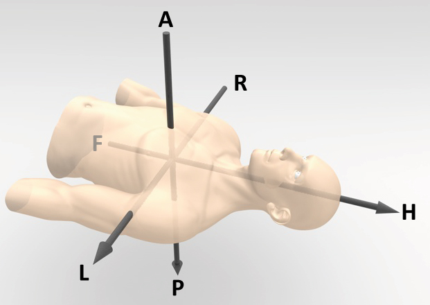
The patient coordinate system is bound to the patient and does not depend on the imaging volume. It is however dependent on the patient position, meaning that when the patient switches his position from supine to prone, the Patient system rotates with him (see below for more information). The axes in the patient coordinate system are expressed in Anterior-Posterior (AP), Right-Left (RL) and Feet-Head (FH) directions (see image below). The units of the coordinates in the ‘RAF’-system are given in mm and it is right handed. The ‘RAF’-system is useful if one wants to compare/overlay the anatomy from different scans.

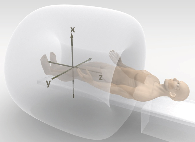
Scanner coordinate system ‘xyz’ [mm]

The scanner coordinate system is bound to the scanner and is the “simplest” system of them all. It is independent of the Patient position/orientation, imaging volume, table movement etc. Its origin is always located in the isocenter of the scanner and it is right-handed. The z-axis is parallel to the bore of the scanner while the y and z axes are perpendicular to it (see image below).

Scanner interface and coordinate systems

Interactions on the scanner interface can influence the coordinate systems. In the following section we describe what parameter and actions change/influence the coordinate systems.

Geometry manipulations on the scanner

Geometry manipulations on the scanner can either be done interactively by moving, rotating or resizing the imaging volume per drag and drop or manually via the parameter in the user interface. Below is a description of parameters/actions and their effect on the coordinate systems.

Shifting the volume/changing offcentre: shifting the imaging volume changes the image offcentre. The offcentre is usually expressed in the ‘RAF’-system and is the distance in mm between the positioning laser mark (set at the beginning of the exam) and the MPS origin. It will also change the MPS offcentre which is the distance in mm between the MPS origin and the isocenter (xyz origin) expressed in MPS coordinates. The offcentre and MPS offcentre is essentially the same vector as long as the table didn’t move (see table movement).

Rotating the volume/changing angulation: rotating the imaging volume changes the imaging angulation. The imaging angulation is given in degrees and specifies a rotation around an axis in the ‘RAF’-system (e.g. an RL-angulation of 10 means a rotation of 10° around the RL axes). The angulation is always in the range of 0°-45°. If the rotation angle becomes larger than 45° the image orientation is changed (e.g. if a transversal slice is rotated more than 45° around the AP-axes it becomes a sagittal slice). Therefore every axis in the MPS-system can be expressed in RL-AP-FH notation (e.g. the readout axes is said to be “parallel” to the RL axes if it is not rotated more than 45° around the AP axis).

Imaging Orientation: The imaging orientation can either be Transversal, Coronal, or Sagital. Resetting this parameter changes the orientation of the MPS system compared to the RAF/xyz-systems.

Fold-over direction: The fold-over direction specifies the phase encoding direction expressed in RL-AP-FH notation. Resetting it changes the orientation of the MPS system compared to the RAF/xyz-systems.

Fatshift direction: Changing the fatshift direction inverts both the readout direction as well as the first phase encoding direction (the MPS system is flipped).

Table movement

During the exam the scanner table might move since the selected imaging volume is too far away from the isocenter. The xyz-system is independent of the table movement and its origin will remain in the isocenter. However the patient system RAF remains fixed with the patient and will move relative to the xyz-system. This means that the origin of the RAF-system will remain at the same anatomy (which corresponds to the laser marker) if the table moves. Or in other words, a slice showing the same anatomy is identical in the RAF system when transformed before and after table movement, but is shifted in the xyz system.

Patient position/orientation

The patient position can either be set as “Head-First” or “Feet-First” while the patient orientation can either be “supine”, “prone”, “right” or “left”. For the patient position/orientation the same goes as for the table movement: The xyz-system is independent of the setting but the patient coordinate system will rotate with the patient. For example in “supine” position the y-axis is equal to the RL-axis, however in “prone” position the y-axes is flipped and corresponds to the LR-axis.

Summary

The image below shows an illustration of all the coordinate systems we can have on the scanner and in MRecon. Furthermore in the table below all the different coordinate systems are expressed in RL-AP-FH notation depending on the imaging parameters, and patient position/orientation.

MPS / REC-systems

Cartesian

Orientation	Fold-Over Dir	Fat Shift	MPS System	REC System
SAG	AP	F	HF-PA-RL	HF-AP-LR
SAG	AP	H	FH-AP-RL	HF-AP-LR
SAG	FH	A	PA-FH-RL	HF-AP-LR
SAG	FH	P	AP-HF-RL	HF-AP-LR
TRA	AP	L	RL-AP-HF	AP-RL-FH
TRA	AP	R	LR-PA-HF	AP-RL-FH
TRA	RL	A	PA-RL-HF	AP-RL-FH
TRA	RL	P	AP-LR-HF	AP-RL-FH
COR	RL	F	HF-LR-PA	HF-RL-AP
COR	RL	H	FH-RL-PA	HF-RL-AP
COR	FH	L	RL-HF-PA	HF-RL-AP
COR	FH	R	LR-FH-PA	HF-RL-AP

Radial

Orientation	Fold-Over Dir	Fat Shift	MPS System	REC System
SAG	N/A	N/A	FH-AP-RL	HF-AP-LR
TRA	N/A	N/A	PA-RL-HF	AP-RL-FH
COR	N/A	N/A	FH-RL-PA	HF-RL-AP

Kooshball

Orientation	Fold-Over Dir	Fat Shift	MPS System	REC System
SAG	N/A	N/A	HF-AP-RL	HF-AP-LR
TRA	N/A	N/A	AP-RL-HF	AP-RL-FH
COR	N/A	N/A	HF-RL-PA	HF-RL-AP

Spiral

Orientation	Fold-Over Dir	Fat Shift	MPS System	REC System
SAG	N/A	N/A	AP-HF-RL	HF-AP-LR
TRA	N/A	N/A	RL-AP-HF	AP-RL-FH
COR	N/A	N/A	RL-HF-PA	HF-RL-AP

EPI

Orientation	Fold-Over Dir	Fat Shift	MPS System	REC System
SAG	AP	A	HF-PA-RL	HF-AP-LR
SAG	AP	P	FH-AP-RL	HF-AP-LR
SAG	FH	F	AP-HF-RL	HF-AP-LR
SAG	FH	H	PA-FH-RL	HF-AP-LR
TRA	AP	A	LR-PA-HF	AP-RL-FH
TRA	AP	P	RL-AP-HF	AP-RL-FH
TRA	RL	R	AP-LR-HF	AP-RL-FH
TRA	RL	L	PA-RL-HF	AP-RL-FH
COR	RL	R	HF-LR-PA	HF-RL-AP
COR	RL	L	FH-RL-PA	HF-RL-AP
COR	FH	F	RL-HF-PA	HF-RL-AP
COR	FH	H	LR-FH-PA	HF-RL-AP

xyz-systems

Patient Position	Patient Orientation	xyz-System
Head First	Supine	PA-RL-FH
Head First	Prone	AP-LR-FH
Head First	Left	LR-PA-FH
Head First	Right	RL-AP-FH
Feet First	Supine	PA-LR-HF
Feet First	Prone	AP-RL-HF
Feet First	Left	LR-AP-HF
Feet First	Right	RL-PA-HF

Coordinate transformations

With MRecon every coordinate system can be transformed into another using the Transform function. Its syntax is:

>> [xT, A] = r.Transform( x, from\_system, to\_system, stack )

or

>> A = r.Transform( from\_system, to\_system, stack )

Input	Description
x	3-dimensional row vector in the source system which is transformed to the target system
from_system	The source system. Possible values are: ‘ijk’, ‘MPS’, ‘MPSpix’, ‘REC’, ‘RAF’, ‘xyz’
to_system	The target system. Possible values are: ‘ijk’, ‘MPS’, ‘MPSpix’, ‘REC’, ‘RAF’, ‘xyz’
stack	(Optional). The transformation is calculated on the geometry of that stack

Output	Description
xT	The transformed vector x
A	The transformation matrix which transforms a coordinate from the source system to the target system

The Transform function will calculate the transformation from the geometry Parameter which are currently stored in the reconstruction object.

Examples

Find the matrix index of the MPS origin

Assume we have the following reconstruction object, with a current data matrix of 288x288x15:

r =

  MRecon with properties:

         Parameter: [1×1 MRparameter]
              Data: [288x288x15 single]
    DataProperties: []

Suppose we want to find the matrix index into r.Data which specifies the pixel lying in the origin of the MPS-system. This means we have to transform the coordinate (0,0,0) from the MPS system to the ijk system (matrix system of the current data matrix):

>> xT = r.Transform( [0,0,0], 'MPS', 'ijk' )

xT =

  144.5000
  144.5000
    8.0000

As expected the resulting index is exactly the center of the data matrix in Matlab matrix notation.

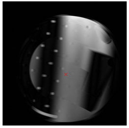
Find the voxel which is in the isocenter

To locate the voxel which lays in the isocenter transform the coordinate (0,0,0) from the xyz-system to the ijk-system:

>> ISO = r.Transform( [0;0;0], 'xyz', 'ijk' )

ISO =

  170.2983
  147.3756
    8.0075

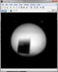
Show the isocenter in the image:

>> figure, imshow( r.Data(:,:,round(ISO(3) )), [] );
>> hold on;
>> plot( ISO(2), ISO(1), 'rx', 'MarkerSize', 8 )

Transform the MPS-system origin to the RAF-system

If we transform the MPS origin to the patient system we get the following:

>> xT = r.Transform( [0;0;0], 'MPS', 'RAF' )

xT =

    -12.0401
    1.2638
    16.8283

This corresponds exactly to the offcentres which are stored in the scan parameter (ap,fh,rl):

>> r.Parameter.Scan.Offcentre

ans =

  1.2638    16.8283    -12.0401

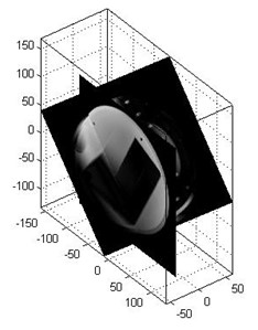
Plot an imaging slice in 3d

Let’s assume we want to plot a slice of our dataset in 3d by transforming it to the patient system RAF:

First select a slice to show in 3d and get the matrix size:

>> slice_nr = 8;
>> siz = size( r.Data );

Create a list of all the pixels in the image (ijk-coordinates):

>> [x,y,z] = ndgrid( 1:siz(1), 1:siz(2), slice_nr);
>> X = [x(:), y(:), z(:)]';

Transform the ijk-coordinates to the RAF system:

>> XT = r.Transform( X, 'ijk', 'RAF' );

Recreate the coordinate grid from the transformed coordinates:

>> xT = reshape(XT(1,:), siz(1),siz(2) );
>> yT = reshape(XT(2,:), siz(1),siz(2) );
>> zT = reshape(XT(3,:), siz(1),siz(2) );

plot the selected slice at the transformed locations in 3D:

>> figure; surf( xT, yT, zT, double(r.Data(:,:,slice_nr)), 'EdgeColor', 'none');
>> colormap(gray);

Repeat the above process to overlay slices from multiple scans:

Reformat a 3D volume to a given geometry

Assume we have two scans: a large 3D volume and a scan with an arbitrary geometry. We now want to fit the geometry of the second scan into the 3D volume and display a reformatted view of the 3D volume.

In the following example with fit an angulated slice into a low resolution SENSE reference scan. The low resolution reformatted slice could afterwards be used to calculate the coil sensitivity maps.

To do that we have to transform the coordinates of the angulated slice into the coordinate system of the refscan. Or in other words we have to transform the ijk-system of the angulated slice to the ijk-system of the refscan. We do that in two steps:

1. Transform the ijk-system of the angulated slice to the RAF-system

2. Transform the RAF-coordinates to the ijk-system of the refscan

We start of y reading and reconstructing the reference scan and the angulated slice:

>> ref = MRecon('refscan.lab');
>> ref.Perform
>> r = MRecon('angulated_slice.lab');
>> r.Perform
>> r.ShowData;

Afterwards we get the transformation matrix which transform the image coordinates of the angulated slice to the RAF-system (A is a 4x4 affine transformation matrix):

>> A = r.Transform('ijk', 'RAF' );

Then we get the transformation matrix which transforms the refscan into the RAF-system (of the first stack):

>> B = ref.Transform('ijk', 'RAF', 1 );

The transformation which transforms the ijk-system of the angulated slice into the ijk-system of the refscan is now given by: B^-1A. We now transform the image coordinates of the angulated slice to the image coordinate system of the refscan:

>> [ x,y,z ] = ndgrid( 1:size(r.Data,1), 1:size(r.Data,2), 1 );
>> X = [x(:), y(:), z(:), ones( size(x(:)))]';
>> Xref = inv(B)\*A\*X;

We now have the coordinates of the angulated slice in the matrix coordinate system of the refscan. All we have to do now is to interpolate the refscan at these positions (we interpolate the second stack which is the bodycoil):

>> ref_slice = interp3( ref.Data(:,:,:,1,1,1,1,2,1), ...
>> Xref(2,:), Xref(1,:), Xref(3,:) );
>> ref_slice = reshape( ref_slice, size(r.Data) );

ref_slice now contains a reformatted slice of the refscan in the geometry of the high resolution scan: